Radiqant

Real estate: correlation between volumes and returns

This analysis will focus on companies in the real estate select sector index, assessing the existence of a correlation between its volumes and subsequent returns.

After the subprime crisis, the Real Estate Select Sector index gradually increased in value, as can be seen in Figure 1.

Figure 1. The figure shows the Real Estate Select Sector index performance since 2005 (source: https://www.investing.com/indices/dj-us-select-real-estate)


We will see if there is a correlation of returns between a short period characterized by an increase in prices and volumes, and an immediately subsequent period marked by an appreciation in the value of shares.

In particular, by taking the first 3 trading days of the month, the following conditions must be met:

  • The total return of the first 3 days must be positive;
  • The daily volumes of the first 3 days must be increasing according to the relation Volumet1 < Volumet2 < Volumet3;
  • The average daily volume of the first 3 days must be higher than the average daily volume of the previous month plus 10%.

Respecting the constraints, let’s see how the stocks behave by entering the market long on day 4 and holding the position for 3 different holding periods: 1, 2 and 3 days.


Ticker

Total Trades

Avg Return 1st Period

Win Ratio 1st Period

Avg Return 2nd Period

Win Ratio 2nd Period

Avg Return 3rd Period

Win Ratio 3rd Period

AMT

4

3,0%

0,75

3,8%

0,75

5,2%

0,75

ARE

2

3,3%

1,00

3,7%

1,00

4,9%

1,00

AVB

3

3,9%

0,67

3,5%

0,67

3,5%

0,67

BXP

4

6,8%

1,00

6,7%

1,00

8,0%

1,00

CBRE

6

2,2%

0,67

2,2%

0,67

2,9%

0,67

CCI

3

2,1%

1,00

2,2%

1,00

1,0%

0,67

DLR

6

5,2%

0,83

5,9%

0,83

5,9%

0,83

DRE

6

2,7%

0,83

2,6%

0,67

3,3%

0,67

EQIX

4

1,1%

0,75

1,2%

0,50

1,1%

0,50

EQR

5

5,1%

1,00

6,9%

1,00

7,6%

1,00

ESS

2

-2,2%

0,50

-2,2%

0,50

-0,3%

0,50

EXR

4

3,7%

0,75

5,1%

1,00

5,9%

1,00

FRT

3

0,0%

0,67

0,8%

0,67

7,1%

0,67

HST

9

-1,2%

0,44

1,3%

0,67

2,1%

0,56

IRM

0

KIM

5

4,0%

0,80

4,5%

0,80

4,5%

0,60

MAA

2

6,5%

1,00

6,1%

1,00

7,1%

1,00

O

5

5,2%

0,80

5,3%

1,00

5,5%

1,00

PEAK

4

6,7%

1,00

8,0%

1,00

7,7%

1,00

PLD

3

5,4%

1,00

5,6%

1,00

6,3%

1,00

PSA

2

8,1%

1,00

8,4%

1,00

6,5%

1,00

REG

3

9,1%

1,00

9,2%

1,00

8,8%

1,00

SBAC

2

2,0%

0,50

1,5%

0,50

0,4%

0,50

SLG

2

12,0%

1,00

13,3%

1,00

13,8%

1,00

SPG

5

9,5%

0,80

13,6%

0,80

11,2%

0,80

UDR

8

3,4%

0,63

5,1%

0,75

6,2%

0,75

VTR

7

4,7%

0,71

5,4%

0,86

6,8%

1,00

WELL

3

6,9%

1,00

6,8%

1,00

7,5%

1,00

WY

4

2,1%

0,75

3,9%

0,75

3,3%

0,75


By analysing the data, the following considerations can be made:

1st Holding Period – One day

  • 1/29 stocks have a WR below 50%;
  • 2/29 have a WR of 50%;
  • 25/29 have a WR above 50%;
  • In total, out of 116 observations resulting in a WR of 82%, only 2 in 19 stocks have a negative average return.

In total, the 116 trades observed produce an average return of 4.3%.


2st Holding Period – Two days

  • 0/29 stocks have a WR below 50%;
  • 3/29 have a WR of 50%;
  • 25/29 have a WR above 50%;
  • In total, out of 116 observations resulting in a WR of 83%, only 1 in 19 stocks has a negative average return 

In total, the 116 trades observed produce an average return of 5%.


3st Holding Period – Three Days

  • 0/29 stocks have a WR below 50%;
  • 3/29 have a WR of 50%;
  • 25/29 have a WR above 50%;
  • In total, out of 116 observations resulting in a WR of 82%, only 1 in 19 stocks has a negative average return.

In total, the 116 trades observed produce an average return of 5.5%.


This settings strategy acquires strength and relevance from the good quantitative data that are derived from and support it. 

However, the one presented here is non fully optimized, but it just represents an idea of how volumes and returns can be correlated.

Giuseppe Ferrulli

CEO, Radiqant
Share on

Other articles

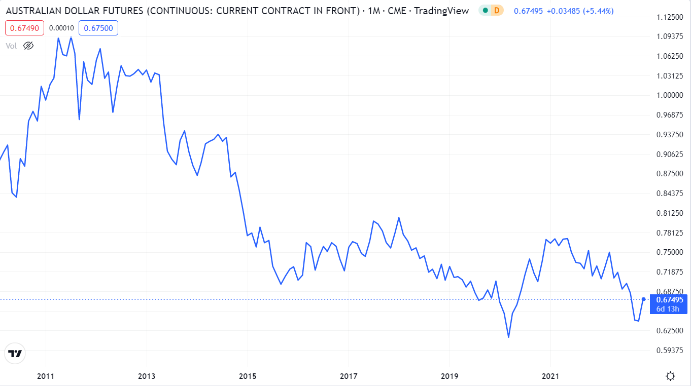
TREND FOLLOWINGIn this analysis we will consider the AUD futures. Dividing the time series starting in 2003, we will look for an entry that breaks a monthly high-open candle formed the same month as the year before.
Mean Reversion In this analysis, we will consider the CAD futures. Dividing the time series starting in 2002, we will look for the existence of a correlation between the various months.