Kinder Morgan Inc (KMI) Time-band Bias

In this analysis we will present an Hourly Bias identified among the US stocks within the S&P500 index.

A Bias is an inefficiency that recurs on the market with a certain frequency, in this case linked to specific time bands. It is a simple analysis, but it can give very useful information, above all if the carried out study is contextualized.

This research is conducted on Kinder Morgan Inc, one of the largest energy infrastructure companies in North America. The company is engaged on several fronts: management of pipelines and terminals that transport natural gas, gasoline, crude oil, carbon dioxide (CO2) and other products; storage of petroleum chemicals; and finally, management of bulk materials such as ethanol, coal, petroleum coke and steel.

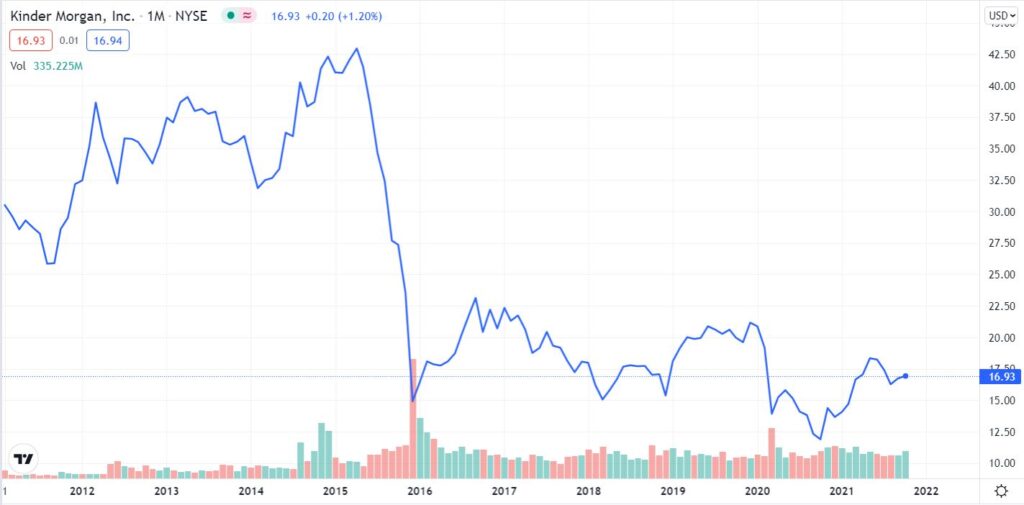
The time series is analysed on an hourly time frame starting on February 11th, 2011, when KMI began trading on the NYSE again, following the largest US private equity-backed IPO offering in history.

Figure 1. Monthly KMI trend (source: https://it.tradingview.com/chart/?symbol=NYSE%3AKMI)

If we exclude the decline in 2015, we can see from the figure that the stock has no particular long-term trend.

Analysing the time slots in search of bias, the following trading hours are taken: 10:00 (NY) – 15:00 (NY).

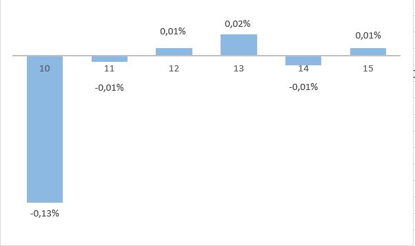
Figure 2. Average return per hour

As we can see from Figure 2, the 10 o’clock hour presents an average return in absolute value much larger than the other analysed hours of the day. In this case the tendency of the 10 o’clock hour is to go short: it has an average return of 0.13% and the number of negative hours has a Win Ratio of 56%.

In an attempt to enhance this bias we will rely on autocorrelations of negative returns. Such time dependence between returns, which is identified by the name of volatility clustering, corresponds to some extent to the behaviour of economic agents that leads to periods of high volatility of negative returns. Indeed, prices move on the basis of agents’ reactions to information streams that often arrive in clusters.

The conditional heteroschedasticity hypothesis presents larger shocks in the case of negative returns. Indeed, in most cases the volatility increases more after bad news and negative returns than after good news and positive returns (levarage effect).

On the basis of the above, we filter out the 10 o’clock hour by identifying the negative increasing returns on the 2 days immediately preceding.

Constraint

As a constraint, we define that the sum of the returns on day t-1 must be less than the difference between the average of the hourly returns recorded on day t-2 and the doubled-standard deviation of the hourly returns on day t-2, as stated in the formula below.

(Σ_i=10:15 xi) _t-1 < ( μ – 2σ) _t-2

x = hourly yields
t = day taken into account
i = 10:15 -> hours taken into account
μ = average hourly yields
σ = Standard deviation of hourly yields

Taking twice the dev.st we filter out and get 5% of the most extreme returns of the normal distribution.

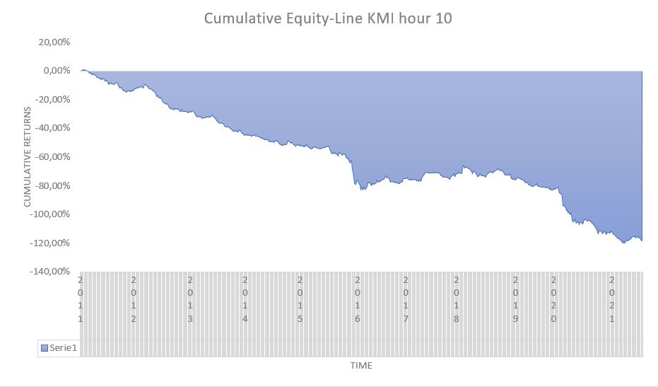
Respecting this constraint, we get an increase in average return from -0.13% to -0.18%, with a Win Ratio of negative hours increasing from 56% to 60% and a Profit Factor of 1,77.

The resulting cumulative equity line will be as shown in the figure below.